Bayesian Changepoint Detection in (Num)Pyro

Posted on Tue 08 June 2021 in probabilistic programming, changepoint detection, Bayesian

Chad Scherrer has a blog post about how to do Bayesian changepoint detection in PyMC3, in the context of detecting changepoint associated with the yearly number of coal mining disasters. Here we will see how to implement the same model in Pyro, a probabilistic programming language and environment using PyTorch as its backend, and also NumPyro, a variant of Pyro with Jax backend. Note that although Pyro and NumPyro support running the computation using GPU, here are we are going to stick with CPU.

Let us start by setting up the necessary packages. For visualization, we are using the standard matplotlib package along with the plotnine package. The reason for plotnine is it allows us to use ggplot2-like syntax for plotting.

%reload_ext autoreload
%autoreload 2
%matplotlib inline

import numpy as np
import pandas as pd

import torch

import pyro
import pyro.infer
import pyro.distributions as pyrodist

import numpyro
import numpyro.infer
import numpyro.distributions as numpyrodist

from jax import random

numpyro.set_platform('cpu')
numpyro.set_host_device_count(4)

import matplotlib.pyplot as plt
from plotnine import *
plt.style.use('seaborn')

Next, let us load and check the data.

# from http://people.reed.edu/~jones/141/Coal.html
coal_df = pd.DataFrame({
    'year': [1851, 1852, 1853, 1854, 1855,
1856, 1857, 1858, 1859, 1860, 1861, 1862, 1863, 1864, 1865, 1866,
1867, 1868, 1869, 1870, 1871, 1872, 1873, 1874, 1875, 1876, 1877,
1878, 1879, 1880, 1881, 1882, 1883, 1884, 1885, 1886, 1887, 1888,
1889, 1890, 1891, 1892, 1893, 1894, 1895, 1896, 1897, 1898, 1899,
1900, 1901, 1902, 1903, 1904, 1905, 1906, 1907, 1908, 1909, 1910,
1911, 1912, 1913, 1914, 1915, 1916, 1917, 1918, 1919, 1920, 1921,
1922, 1923, 1924, 1925, 1926, 1927, 1928, 1929, 1930, 1931, 1932,
1933, 1934, 1935, 1936, 1937, 1938, 1939, 1940, 1941, 1942, 1943,
1944, 1945, 1946, 1947, 1948, 1949, 1950, 1951, 1952, 1953, 1954,
1955, 1956, 1957, 1958, 1959, 1960, 1961, 1962],
    'count': [4,
5, 4, 1, 0, 4, 3, 4, 0, 6, 3, 3, 4, 0, 2, 6, 3, 3, 5, 4, 5, 3,
1, 4, 4, 1, 5, 5, 3, 4, 2, 5, 2, 2, 3, 4, 2, 1, 3, 2, 2, 1, 1,
1, 1, 3, 0, 0, 1, 0, 1, 1, 0, 0, 3, 1, 0, 3, 2, 2, 0, 1, 1, 1,
0, 1, 0, 1, 0, 0, 0, 2, 1, 0, 0, 0, 1, 1, 0, 2, 3, 3, 1, 1, 2,
1, 1, 1, 1, 2, 4, 2, 0, 0, 0, 1, 4, 0, 0, 0, 1, 0, 0, 0, 0, 0,
1, 0, 0, 1, 0, 1],
})

plt.bar(coal_df['year'], coal_df['count'])

<BarContainer object of 112 artists>

png

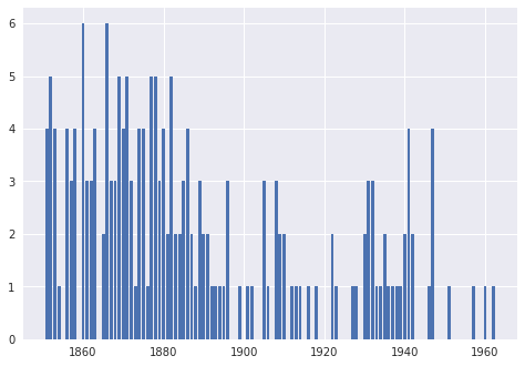
So we confirm that we are using the same data as the one used by Chad Scherrer. We are now ready for the model; for simplicity, we use the same model as used by Chad Scherrer:

$$ \begin{align*} T &\sim \mathrm{Uniform}(1860, 1960) \\ \mu_0 &\sim \mathrm{Normal}^+(0, 4) \\ \mu_1 &\sim \mathrm{Normal}^+(0, 4) \\ n_t &\sim \mathrm{Poisson}(\mu_{[t > T]}) \end{align*} $$

We are ready to implement this model in Pyro. In Pyro, a model is implemented as a function with the necessary calls to some Pyro primitives. More information is available here.

def changepoint_model_pyro(year, count):
    # point where distribution changes
    T = pyro.sample('T', pyrodist.Uniform(1860, 1960))
    mu0 = pyro.sample('mu0', pyrodist.HalfNormal(scale=4.))
    mu1 = pyro.sample('mu1', pyrodist.HalfNormal(scale=4.))

    num_years = len(year)
    with pyro.plate('num_years', num_years) as index:
        mu = mu1 * (year[index] > T) + mu0 * (year[index] <= T)

        pyro.sample('obs', pyrodist.Poisson(mu), obs=count[index])

Let us now do inference. In particular, here we are interested in the posterior distributions for $T, \mu_0, \mu_1$. In the original blog post, inference is done using Markov Chain Monte Carlo (MCMC) as implemented in PyMC3; we are going to follow the MCMC route also and in particular we use the NUTS sampler implemented in Pyro. As a note, Pyro also supports an alternative way to do inference by using stochastic variational inference, more details on how to do this here, here, here, and here.

For our inference, we are going to generate 500 samples for warmup, and 500 samples for the actual inference. Four chains will be generated; in Pyro, a CPU core will be dedicated for each chain.

num_samples = 500
warmup_steps = 500
num_chains = 4

nuts_kernel = pyro.infer.NUTS(changepoint_model_pyro)
mcmc = pyro.infer.MCMC(nuts_kernel,
                       num_samples=num_samples,
                       warmup_steps=warmup_steps,
                       num_chains=num_chains)
mcmc.run(torch.tensor(coal_df['year'].to_numpy(), dtype=torch.float), torch.tensor(coal_df['count'].to_numpy(), dtype=torch.float))
mcmc.summary(prob=0.5)

                mean       std    median     25.0%     75.0%     n_eff     r_hat
         T   1890.14      2.39   1890.45   1889.52   1892.00    114.73      1.05
       mu0      3.17      0.30      3.14      2.90      3.29     49.39      1.09
       mu1      0.94      0.11      0.94      0.85      1.00    165.78      1.02

Number of divergences: 0

On my machine with Intel Xeon E5-2680 v4, inference takes quite slow to run, even with a total of only 1000 samples. In particular, generating the samples seems relatively time consuming, taking about 2-3 seconds per sample.

We also see some summary statistics of the parameters based on the MCMC run. The first to note is that the number of divergences is zero, which indicates no parameters diverge. This is a good sign. On the other hand, the r_hat values are above 1.00, which indicates that convergence has not been reached. Also the effective sample sizes (n_eff) seem pretty low, ranging from 80 to 116 out of the 500 post-warmup samples.

So it seems we need more samples. But on the other hand, the above run was quite slow. Would using NumPyro instead help? Let us check it out.

As you can see below, translating a Pyro model to NumPyro is pretty straightforward, we just need to make sure that the appropriate packages are used, and in NumPyro, we need to pass Jax's pseudorandom number generator key as the first argument when running MCMC. Let us see how this runs.

def changepoint_model_numpyro(year, count):
    # point where distribution changes
    T = numpyro.sample('T', numpyrodist.Uniform(1860, 1960))
    mu0 = numpyro.sample('mu0', numpyrodist.HalfNormal(scale=4.))
    mu1 = numpyro.sample('mu1', numpyrodist.HalfNormal(scale=4.))

    num_years = len(year)
    with numpyro.plate('num_years', num_years):
        mu = mu1 * (year > T) + mu0 * (year <= T)

        numpyro.sample('obs', numpyrodist.Poisson(mu), obs=count)

num_samples = 10000
warmup_steps = 10000

nuts_kernel = numpyro.infer.NUTS(changepoint_model_numpyro)
mcmc = numpyro.infer.MCMC(
    nuts_kernel,
    num_samples=num_samples,
    num_warmup=warmup_steps,
    num_chains=num_chains)
rng_key = random.PRNGKey(0)
mcmc.run(rng_key, coal_df['year'].to_numpy(), coal_df['count'].to_numpy())
mcmc.print_summary()

                mean       std    median      5.0%     95.0%     n_eff     r_hat
         T   1890.30      2.43   1890.52   1886.00   1893.04   1324.71      1.00
       mu0      3.13      0.29      3.12      2.67      3.61   1499.55      1.00
       mu1      0.94      0.12      0.93      0.74      1.14   1535.97      1.00

Number of divergences: 0

Wow, even with 20x the number of samples (10,000 warmup samples and 10,000 samples for inference), the code runs much faster, finishing in around a minute including the JIT compilation step in the beginning. With these many samples, we see from r_hat that they seem to have reached convergence. Still, the effective sample sizes from n_eff seem low, corresponding to less than 20% of the 10,000 actual samples. One consideration is re-evaluating the use of the HalfNormal distribution as priors for $\mu_0$ and $\mu_1$. In particular, for the Poisson distribution, the conjugate prior is given by a Gamma distribution. If we use Gamma priors for $\mu_0$ and $\mu_1$, would we see a bump in n_eff?

Let us evaluate it by considering a revised model:

$$ \begin{align*} T &\sim \mathrm{Uniform}(1860, 1960) \\ \mu_0 &\sim \mathrm{Gamma}(5, 1) \\ \mu_1 &\sim \mathrm{Gamma}(5, 1) \\ n_t &\sim \mathrm{Poisson}(\mu_{[t > T]}) \end{align*} $$

We implement and run this model below.

def changepoint_model_numpyro(year, count):
    # point where distribution changes
    T = numpyro.sample('T', numpyrodist.Uniform(1860, 1960))
    mu0 = numpyro.sample('mu0', numpyrodist.Gamma(5.))
    mu1 = numpyro.sample('mu1', numpyrodist.Gamma(5.))

    num_years = len(year)
    with numpyro.plate('num_years', num_years):
        mu = mu1 * (year > T) + mu0 * (year <= T)

        numpyro.sample('obs', numpyrodist.Poisson(mu), obs=count)

num_samples = 10000
warmup_steps = 10000

nuts_kernel = numpyro.infer.NUTS(changepoint_model_numpyro)
mcmc = numpyro.infer.MCMC(
    nuts_kernel,
    num_samples=num_samples,
    num_warmup=warmup_steps,
    num_chains=num_chains)
rng_key = random.PRNGKey(0)
mcmc.run(rng_key, coal_df['year'].to_numpy(), coal_df['count'].to_numpy())
mcmc.print_summary()

                mean       std    median      5.0%     95.0%     n_eff     r_hat
         T   1890.01      2.46   1890.26   1886.01   1892.93   2165.32      1.00
       mu0      3.18      0.29      3.16      2.69      3.64   2270.01      1.00
       mu1      0.98      0.12      0.98      0.79      1.19   2240.78      1.00

Number of divergences: 0

Yes, we do manage to see a bump in n_eff to above 20% of the total samples. Not great, but we settle with this for now.

In the next group of cells, we are going to visualize the posterior distributions for the parameters based on the samples. Let us first get the actual samples and store them in a pandas DataFrame.

hmc_samples = mcmc.get_samples(group_by_chain=True)

sample_dfs = []
for chain_idx in range(num_chains):
    df = pd.DataFrame({
        'T': hmc_samples['T'][chain_idx],
        'mu0': hmc_samples['mu0'][chain_idx],
        'mu1': hmc_samples['mu1'][chain_idx],
        'sample_index': np.arange(num_samples),
    })
    df['chain'] = chain_idx + 1
    sample_dfs.append(df)

sample_df = pd.concat(sample_dfs)

Let us visualize the distributions and plot the trace of samples. We do this for each chain.

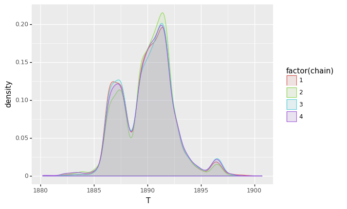
First, the plots for $T$.

(
    ggplot(sample_df, aes(x='T', color='factor(chain)', fill='factor(chain)')) + geom_density(alpha=0.1)
)

png

<ggplot: (8744344050698)>

(
    ggplot(sample_df, aes(x='sample_index', y='T', color='factor(chain)', fill='factor(chain)')) + geom_line()
)

png

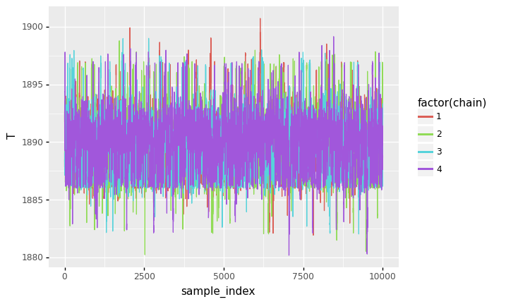
<ggplot: (8744343967368)>

Next the plots for $\mu_0$.

(
    ggplot(sample_df, aes(x='mu0', color='factor(chain)', fill='factor(chain)')) + geom_density(alpha=0.1)
)

png

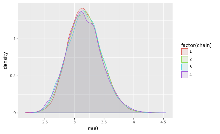
<ggplot: (8744343942813)>

(
    ggplot(sample_df, aes(x='sample_index', y='mu0', color='factor(chain)', fill='factor(chain)')) + geom_line()
)

png

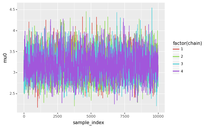
<ggplot: (8744343868314)>

And finally, the plots for $\mu_1$.

(
    ggplot(sample_df, aes(x='mu1', color='factor(chain)', fill='factor(chain)')) + geom_density(alpha=0.1)
)

png

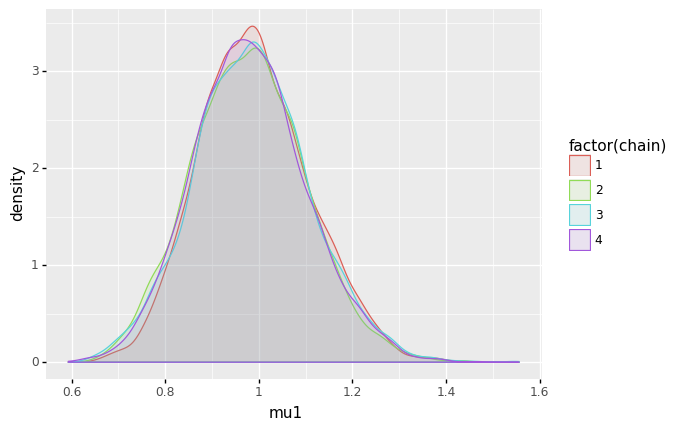
<ggplot: (8744343839407)>

(
    ggplot(sample_df, aes(x='sample_index', y='mu1', color='factor(chain)', fill='factor(chain)')) + geom_line()
)

png

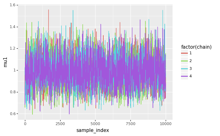
<ggplot: (8744343770902)>

Some observations:

For $T$, we roughly see 3 modes in the posterior distribution. The highest mode is around 1891-1892.
For $\mu_0$ and $\mu_1$, the posterior distributions seem to be unimodal and symmetric. For $\mu_0$, the mode is slightly above 3 (meaning a rate of roughly 3 mining disasters per year), while for $\mu_1$, the mode is slightly below 1 (meaning a rate of slightless than 1 mining disaster per year).

Last but not least, we see at least for this particular problem, NumPyro is much faster than Pyro. For future exploration, we can explore ways to reparametrize the model to increase n_eff further.