Kolm and Ritter (2018)
Posted on Sat 12 October 2019 in reinforcement learning
%reload_ext autoreload
%autoreload 2
%matplotlib inline
In an SSRN paper, Petter Kolm and Gordon Ritter present the application of reinforcement learning for model-free European call option hedging. Unfortunately, there does not seem to be any code made available to accompany this paper. Here we try to replicate the results of the paper.
Let us first import the necessary packages.
import numpy as np
import scipy.stats as si
import matplotlib.pyplot as plt
from catboost import CatBoostRegressor
from tqdm import tqdm, tqdm_notebook
from functools import partial
from joblib import Parallel, delayed
import math
import gym
plt.style.use('seaborn')
import seaborn as sns
Next, we implement functions to calculate the price and delta for a European option (call/put, credit to Aaron Schlegel).
def euro_vanilla(S, K, T, r, sigma, option = 'call'):

    #S: spot price
    #K: strike price
    #T: time to maturity
    #r: interest rate
    #sigma: volatility of underlying asset

    if T > 0:
        d1 = (np.log(S / K) + (r + 0.5 * sigma ** 2) * T) / (sigma * np.sqrt(T))
        d2 = (np.log(S / K) + (r - 0.5 * sigma ** 2) * T) / (sigma * np.sqrt(T))

        if option == 'call':
            result = (S * si.norm.cdf(d1, 0.0, 1.0) - K * np.exp(-r * T) * si.norm.cdf(d2, 0.0, 1.0))
        if option == 'put':
            result = (K * np.exp(-r * T) * si.norm.cdf(-d2, 0.0, 1.0) - S * si.norm.cdf(-d1, 0.0, 1.0))
    else:
        if option == 'call':
            result = S - K if S > K else 0
        if option == 'put':
            result = K - S if K > S else 0

    return result

def euro_vanilla_delta(S, K, T, r, sigma, option = 'call'):

    #S: spot price
    #K: strike price
    #T: time to maturity
    #r: interest rate
    #sigma: volatility of underlying asset

    if T > 0:
        d1 = (np.log(S / K) + (r + 0.5 * sigma ** 2) * T) / (sigma * np.sqrt(T))
        d2 = (np.log(S / K) + (r - 0.5 * sigma ** 2) * T) / (sigma * np.sqrt(T))

        delta = si.norm.cdf(d1, 0.0, 1.0)

        if option == 'call':
            return delta
        if option == 'put':
            return delta - 1.0
    else:
        return 0.0
We also need to simulate our underlying prices, which we assume to be a geometric Brownian motion (see this StackOverflow post for details).
def simulate_GBM(S0, mu, sigma, dt, T, N, numts):
    # S0: starting level
    # mu: drift
    # sigma: volatility
    # dt: the timestep unit
    # T: end time
    # N: the number of elements in the time series
    # numts: number of time series to generate

    t = np.linspace(0, T, N)

    W = np.random.randn(numts, N)
    W = np.cumsum(W, axis=1)*np.sqrt(dt) ### standard brownian motion ###
    X = (mu-0.5*sigma**2)*t + sigma*W
    S = S0*np.exp(X) ### geometric brownian motion ###

    return S, t

def simulate_prices(S0, mu, sigma, T, D, numts):
    N = T * D + 1
    dt = 1 / D

    return simulate_GBM(S0, mu, sigma, dt, T, N, numts)
Let us test our price simulation function by generating a sequence of prices and plotting them.
prices, t = simulate_prices(100, 0, 0.01, 10, 5, 10)
plt.plot(t, prices[5,:])
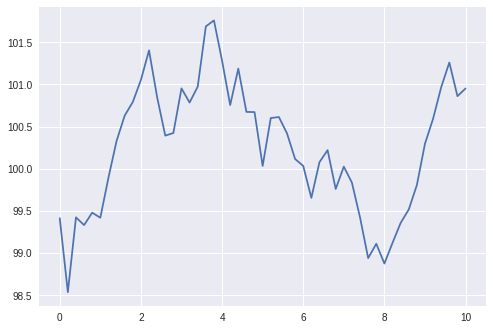
Looks reasonable. Now we are ready to implement our simulation environment. We follow the interface of OpenAI gym's environment. We also implement the transaction cost calculator, following the formula used in the paper:
When this calculator is passed to our environment, the costs of our transactions will be included in the reward. The basic reward follows equation (10) in the paper:
Our state space consists of
- stock price
- time to expiry
- number of shares held
Our action space is a non-negative integer below 100, to reflect the number of shares to hold (short) for the next time step. Here, since we assume we are long the call option, the stock position is going to be always short.
In the environment, we keep track of the evolution of the following:
- stock prices
- option prices
- number of shares held short
- PnL for stock and option
- cash and transaction cost
class BasicCostCalculator:
    def __init__(self, tick_size, multiplier):
        self.tick_size = tick_size
        self.multiplier = multiplier

    def __call__(self, n):
        n = np.abs(n)
        return self.multiplier * self.tick_size * (n + 0.01 * n * n)

class BSMEnv(gym.Env):
    def __init__(self, S0, K, r, sigma, T, D, kappa, cost_calculator=None):
        # S0: starting level
        # K: strike price of the option
        # r: interest rate
        # sigma: volatility
        # T: number of days
        # D: number of hedging periods in a day
        # kappa: risk-aversion parameter
        # cost_calculator (optional): calculator to use for transaction costs

        self.S0 = S0
        self.K = K
        self.r = r
        self.sigma = sigma
        self.T = T
        self.D = D
        self.kappa = kappa

        self.prices = None
        self.t = None
        self.idx = None
        self.num_shares = 0
        self.opt_prices = None
        self.cost_calculator = cost_calculator

        self.action_space = gym.spaces.Discrete(100)
        self.observation_space = gym.spaces.Tuple((
            gym.spaces.Box(0., np.inf, [1], dtype=np.float64),
            gym.spaces.Box(0., T, [1], dtype=np.float64),
            gym.spaces.Discrete(100),
        ))

    def reset(self, prices=None, time=None):
        if prices is None:
            prices, time = simulate_prices(self.S0, 0.0, self.sigma, self.T, self.D, 1)
            prices = prices[0,:]

        self.prices = prices
        self.t = time
        self.idx = 0
        self.num_shares = 0
        self.opt_prices = [euro_vanilla(price, self.K, self.T - tm, self.r, self.sigma, 'call') for price, tm in zip(self.prices, self.t)]
        self.deltas = [euro_vanilla_delta(price, self.K, self.T - tm, self.r, self.sigma, 'call') for price, tm in zip(self.prices, self.t)]
        self.opt_pnl = 100 * np.diff(self.opt_prices)
        self.stock_pnl = np.zeros(self.T * self.D)
        self.num_shares_hist = np.zeros(self.T * self.D)
        self.cash_hist = np.zeros(self.T * self.D)
        self.cost_hist = np.zeros(self.T * self.D)
        self.cash = -self.opt_pnl[0]
        self.cash_hist[0] = self.cash
        state = (self.prices[0], self.T, self.num_shares)

        return state

    def step(self, action):
        # buy back the short
        self.cash -= self.prices[self.idx] * self.num_shares

        num_shares_delta = action - self.num_shares
        self.num_shares = action
        self.cash += self.prices[self.idx] * self.num_shares
        self.num_shares_hist[self.idx] = self.num_shares
        self.cash_hist[self.idx] = self.cash
        self.stock_pnl[self.idx] = (self.prices[self.idx] - self.prices[self.idx+1]) * action

        state_next = (self.prices[self.idx+1], self.T - self.t[self.idx+1], self.num_shares)

        d_wealth = self.opt_pnl[self.idx] + self.stock_pnl[self.idx]
        reward = d_wealth - 0.5 * self.kappa * d_wealth * d_wealth
        if self.cost_calculator:
            cost = self.cost_calculator(num_shares_delta)
            self.cost_hist[self.idx] = cost
            reward -= cost

        info = {
            'opt_pnl': self.opt_pnl[self.idx],
            'stock_pnl': self.stock_pnl[self.idx],
            'cost': cost if self.cost_calculator else 0.,
        }

        self.idx += 1
        done = self.idx == self.T * self.D

        return state_next, reward, done, info
With the environment defined, we can implement our hedging agent. First we define an abstract class Hedger for our hedging agent. In this class, we define a collection of abstract functions that will be invoked by our simulator. The main hedging function is hedge().
class Hedger:
    def __init__(self):
        pass

    def eval(self):
        pass

    def train(self):
        pass

    def on_batch_start(self):
        pass

    def on_batch_end(self):
        pass

    def on_episode_start(self):
        pass

    def on_episode_end(self, env):
        pass

    def on_step_start(self):
        pass

    def on_step_end(self, state, reward, info):
        pass

    def hedge(self, state):
        pass
Next we have the hedger implementing the standard Black-Scholes-Merton hedging: BSMHedger. This hedger uses the option's delta to determine how many shares to use for hedging, calling euro_vanilla_delta() defined above to calculate the option's delta.
class BSMHedger(Hedger):
    def __init__(self, K, r, sigma, opt_type):
        self.K = K
        self.r = r
        self.sigma = sigma
        self.opt_type = opt_type

    def hedge(self, state):
        stock_price, time_to_expire, _ = state
        return np.around(100 * euro_vanilla_delta(stock_price,
                                                  self.K,
                                                  time_to_expire,
                                                  self.r,
                                                  self.sigma,
                                                  self.opt_type))
Last but not least, we have our reinforcement-learning hedger. The key member of the hedger is model; model is a model of the Q function, i.e. the mapping between a state-action pair to the corresponding value; it represents the value of taking the action given a particular state. In a given state, the policy then is to select the action with the maximal value given by the Q function when combined with the given state.
The hedger can be in training mode or evaluation mode. In the training mode, we try to learn model while in the evaluation mode, the hedger applies the trained model to decide the hedging action. Before model is learned (initialized), the hedger always takes random actions, while after initialization, the hedger can perform \(\epsilon\)-greedy exploration of the actions during training. At the end of each batch, we fit model based on the rewards obtained in that batch.
In the paper, there is not much detail about what they use as model, besides the fact that it is a nonlinear regression model. Here, we use the catboost regressor from the catboost package, but the hedger interface itself is agnostic to this detail as long as it can call the sklearn API (fit() and predict()) on model.
We note that the procedure done here is somewhat similar to the one described in Ernst, et al (2005).
class RLHedger(Hedger):
    def __init__(self, model, eps, gamma):
        self.model = model
        self.initialized = False
        self.eps = eps
        self.gamma = gamma

        self.state_prev = None
        self.action_prev = None
        self.training = True

        self.X_pred = np.zeros((101, 4))
        for i in range(0, 101):
            self.X_pred[i,3] = i

        self.X = []
        self.y = []

    def eval(self):
        self.training = False

    def train(self):
        self.training = True

    def on_batch_start(self):
        if self.training:
            self.X = []
            self.y = []

    def on_batch_end(self):
        if self.training:
            self.model.fit(np.array(self.X), np.array(self.y).reshape(-1))
            self.initialized = True

    def on_step_end(self, state_next, reward, info):
        if self.training:
            x = list(self.state_prev) + [self.action_prev]
            y = reward

            if self.initialized:
                action, q = self.get_action(state_next)
                y += self.gamma * q

            self.X.append(x)
            self.y.append(y)

    def get_action(self, state):
        self.X_pred[:,:3] = np.array(list(state))

        preds = self.model.predict(self.X_pred)
        idx = np.argmax(preds)
        action = self.X_pred[idx, 3]
        q = preds[idx]

        return action, q

    def hedge(self, state):
        self.state_prev = state

        if not self.initialized or (self.training and np.random.rand() < self.eps[self.eps_idx]):
            action = np.random.randint(0, 101)
        else:
            action, _ = self.get_action(state)

        self.action_prev = action
        return action
We are now ready to implement functions for running our simulations. First, we implement the function to run a specific episode.
def run_episode(episode_idx, env, model, eps, gamma):
    hedger = RLHedger(model, eps, gamma)
    hedger.on_episode_start()
    state = env.reset()
    done = False

    while not done:
        hedger.on_step_start()
        action = hedger.hedge(state)
        state, reward, done, info = env.step(action)
        hedger.on_step_end(state, reward, info)

    hedger.on_episode_end(env)

    return np.stack(hedger.X), np.stack(hedger.y)
Note that there are no dependencies between episodes. We can take advantage of this property and parallelize run_episode() to speed up training. This is done in run_training() below.
def run_training(env, hedger, eps, gamma, nbatches, nepisodes):
    for batch_idx in tqdm_notebook(range(nbatches)):
        hedger.on_batch_start()
        result = Parallel(n_jobs=8)(delayed(partial(run_episode, env=env, model=hedger.model, eps=eps[batch_idx], gamma=gamma))(i) for i in range(nepisodes))

        X = []
        y = []
        for idx in range(nepisodes):
            X_curr, y_curr = result[idx]
            X.append(X_curr)
            y.append(y_curr)

        X_arr = np.concatenate(X, axis=0)
        y_arr = np.concatenate(y, axis=0)

        hedger.X = X_arr
        hedger.y = y_arr

        hedger.on_batch_end()
We also implement the out-of-sample testing function, run_test(). One difference here is that we run the simulation for both the trained reinforcement-learning hedger and the Black-Scholes-Merton hedger. In this function, we also collect the PnL and transaction-cost history of each episode. This function can potentially be parallelized, but we do not do that here.
def run_test(env, hedger, env_ref, hedger_ref, nepisodes):
    pnls = []
    pnls_ref = []
    costs = []
    costs_ref = []
    pnls_info = []
    pnls_info_ref = []

    hedger.eval()
    hedger_ref.eval()
    for episode_idx in tqdm_notebook(range(nepisodes)):
        state = env.reset()
        hedger.on_episode_start()
        done = False
        pnl = 0
        cost = 0
        pnl_list = []

        while not done:
            hedger.on_step_start()
            action = hedger.hedge(state)
            state, reward, done, info = env.step(action)
            pnl_curr = info['opt_pnl'] + info['stock_pnl'] - info['cost']
            pnl_list.append(pnl_curr)
            pnl += pnl_curr
            cost += info['cost']
            hedger.on_step_end(state, reward, info)

        hedger.on_episode_end(env)
        pnls.append(pnl)
        costs.append(cost)
        pnls_info.append(pnl_list)

        state = env_ref.reset(env.prices, env.t)
        hedger_ref.on_episode_start()
        done = False
        pnl = 0
        cost = 0
        pnl_list = []

        while not done:
            hedger_ref.on_step_start()
            action = hedger_ref.hedge(state)
            state, reward, done, info = env_ref.step(action)
            pnl_curr = info['opt_pnl'] + info['stock_pnl'] - info['cost']
            pnl_list.append(pnl_curr)
            pnl += pnl_curr
            cost += info['cost']
            hedger_ref.on_step_end(state, reward, info)

        hedger_ref.on_episode_end(env_ref)
        pnls_ref.append(pnl)
        costs_ref.append(cost)
        pnls_info_ref.append(pnl_list)

    return pnls, pnls_ref, costs, costs_ref, pnls_info, pnls_info_ref
Training
Finally, we are ready to train our reinforcement-learning hedger. First we setup some constants, most of which follow what are used in the paper.
NBATCHES = 5
NEPISODES = 15000
NEPISODES_TEST = 10000
T = 10
D = 5
S0 = 100
SIGMA = 0.01
KAPPA = 0.1
GAMMA = 0.9
EPS = [0.1, 0.09, 0.08, 0.07, 0.06]
TICK_SIZE = 0.1
MULTIPLIER = 5.
We first train the hedger when there are no transaction costs.
env = BSMEnv(S0, S0, 0, SIGMA, T, D, KAPPA)
model = CatBoostRegressor(thread_count=8, verbose=False)
hedger = RLHedger(model, EPS, GAMMA)

run_training(env, hedger, EPS, GAMMA, NBATCHES, NEPISODES)
Then we train the hedger with transaction costs.
env_cost = BSMEnv(S0, S0, 0, SIGMA, T, D, KAPPA, cost_calculator=BasicCostCalculator(tick_size=TICK_SIZE, multiplier=MULTIPLIER))
model_cost = CatBoostRegressor(thread_count=8, verbose=False)
hedger_cost = RLHedger(model_cost, EPS, GAMMA)

run_training(env_cost, hedger_cost, EPS, GAMMA, NBATCHES, NEPISODES)
Out-of-sample testing
Let us now evaluate the hedgers we trained with out-of-sample cases. First we setup the reference Black-Scholes-Merton hedger, and the environments for testing: one environment for our trained hedger and one environment for the reference hedger.
hedger_ref = BSMHedger(S0, 0, SIGMA, 'call')

env = BSMEnv(S0, S0, 0, SIGMA, T, D, KAPPA)
env_ref = BSMEnv(S0, S0, 0, SIGMA, T, D, KAPPA)
env_cost = BSMEnv(S0, S0, 0, SIGMA, T, D, KAPPA, cost_calculator=BasicCostCalculator(tick_size=TICK_SIZE, multiplier=MULTIPLIER))
env_ref_cost = BSMEnv(S0, S0, 0, SIGMA, T, D, KAPPA, cost_calculator=BasicCostCalculator(tick_size=TICK_SIZE, multiplier=MULTIPLIER))
With those setup, we can run the out-of-sample simulations for both the no-transaction-cost and the with-transaction-cost cases.
pnls, pnls_ref, costs, costs_ref, pnls_info, pnls_info_ref = run_test(env, hedger, env_ref, hedger_ref, NEPISODES_TEST)
pnls_cost, pnls_ref_cost, costs_cost, costs_ref_cost, pnls_info_cost, pnls_info_ref_cost = run_test(env_cost, hedger_cost, env_ref_cost, hedger_ref, NEPISODES_TEST)
No transaction costs
We first consider the results in the no-transaction-costs case. We plot the density estimates of the total PnLs in both cases. Below we see that both are centered at zero, with the RLHedger case having slightly fatter tail. Performing the Welch two-sample t-test, we find that the means of the two cases are not statistically significantly different.
sns.kdeplot(pnls, label='RLHedger')
sns.kdeplot(pnls_ref, label='BSMHedger')
plt.legend()
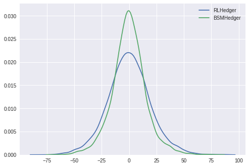
si.ttest_ind(pnls, pnls_ref, equal_var=False)
Ttest_indResult(statistic=-0.005393764800999482, pvalue=0.9956964757476952)
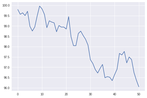
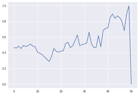
Let us dig into a specific episode. We first plot the stock prices for this episode.
plt.plot(env.prices)
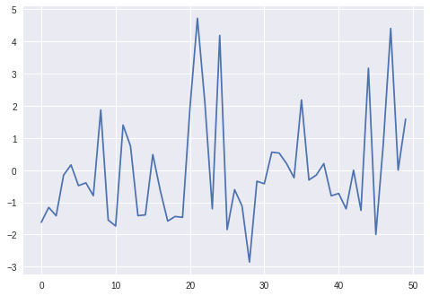
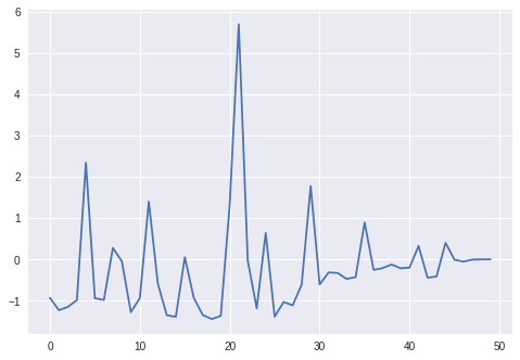
Next we print out the total PnLs and plot the evolution of the PnLs for both RLHedger and BSMHedger. In both cases, there are some small residual total PnLs.
plt.plot(env.opt_pnl + env.stock_pnl)
print(np.sum(env.opt_pnl + env.stock_pnl))
-1.0714312643296595
plt.plot(env_ref.opt_pnl + env_ref.stock_pnl)
print(np.sum(env_ref.opt_pnl + env_ref.stock_pnl))
-11.22226031466913
Next we compare the evolution of the number of shares held short by the RLHedger and the delta of the option. Qualitatively, they look similar.
plt.plot(env.num_shares_hist)
plt.plot(env.deltas)
With transaction costs
Now we consider the case with transaction costs. Looking at the density estimates of the total PnLs, we clearly see a significant difference, and indeed this is also verified by the Welch two-sample t-test (p value 0.0).
sns.kdeplot(pnls_cost, label='RLHedger')
sns.kdeplot(pnls_ref_cost, label='BSMHedger')
plt.legend()
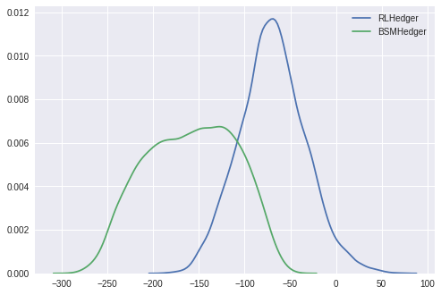
si.ttest_ind(pnls_cost, pnls_ref_cost, equal_var=False)
Ttest_indResult(statistic=147.77669475319246, pvalue=0.0)
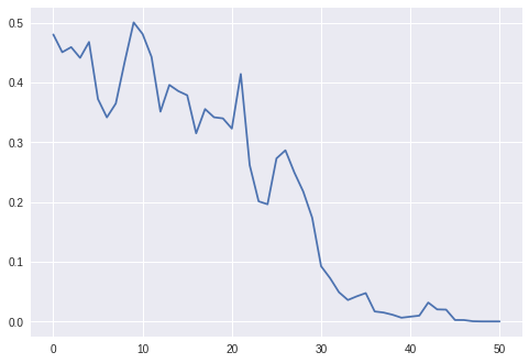
Unlike in the paper, we do find the realized volatility of the PnLs are significantly different for the two cases.
vols_cost = [np.std(x) for x in pnls_info_cost]
vols_ref_cost = [np.std(x) for x in pnls_info_ref_cost]
sns.kdeplot(vols_cost, label='RLHedger')
sns.kdeplot(vols_ref_cost, label='BSMHedger')
plt.legend()
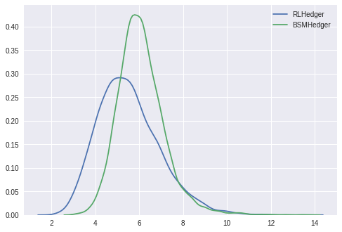
si.ttest_ind(vols_cost, vols_ref_cost, equal_var=False)
Ttest_indResult(statistic=-31.544498387590423, pvalue=8.290086183138852e-213)
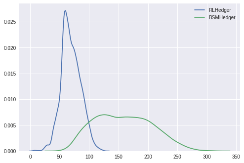
Next we show the density estimates of the total costs. It is clear that the costs for the BSMHedger is significantly higher compared to those for the RLHedger.
sns.kdeplot(costs_cost, label='RLHedger')
sns.kdeplot(costs_ref_cost, label='BSMHedger')
plt.legend()
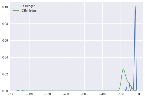
Similar to the paper, we also compute and plot the density estimates of the t-statistics of the PnLs in both cases. The plot shows that the PnLs in the BSMHedger case are more significantly different from zero compared to the PnLs in the RLHedger case.
tstats_cost = si.ttest_1samp(pnls_info_cost, 0.0)
tstats_ref_cost = si.ttest_1samp(pnls_info_ref_cost, 0.0)
sns.kdeplot(tstats_cost[0], label='RLHedger')
sns.kdeplot(tstats_ref_cost[0], label='BSMHedger')
plt.legend()
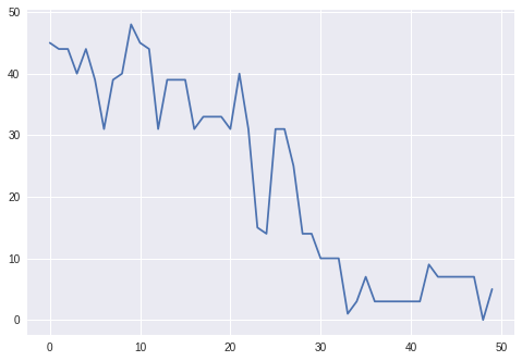
Next we consider a particular episode, in particular, comparing the number of shares held short versus the delta for the RLHedger case. Here we see that the RLHedger case performs the hedging more gradually compared to what is suggested by the delta; for instance, in the beginning, even though delta is higher (around 0.5 since in the beginning the option is at the money), the RLHedger starts with shorting around 20 shares of stock.
plt.plot(env_cost.num_shares_hist)
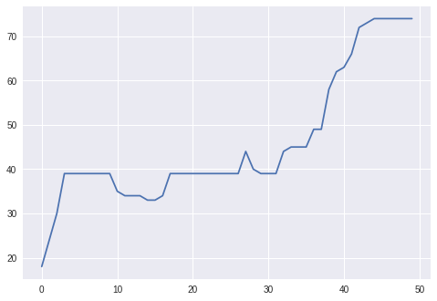
plt.plot(env_cost.deltas)
Saving models
Let us now save the learned catboost models.
hedger.model.save_model('catboost_nocost')
hedger_cost.model.save_model('catboost_cost')